Too Much Idle | OpenGL FDTD Tutorial: Episode 1

Welcome to the first episode of my tutorial to implement real-time physical modelling synthesis on the GPU, using C++ and OpenGL shaders. More context can be found in this introduction.

We’re gonna focus on how to set up OpenGL to run the simulation, giving some details about the physical model we want to implement.
In the context of the full [but small] project, this means looking at two files only:

main.cpp [first part]
openGL_functions.h

The main file contains the C++ initialization code, while the header file has all the prototypes of the functions that wrap the standard OpenGL calls; the trick lies in what we tell the standard functions to do. The actual implementations of these wrappers will be discussed in Episode 3

DISCLAIMER!!!
This tutorial is not meant as an introduction to OpenGL C++ programming,
nor the code snippets are supposed to be tested one by one in an incremental way!
Here I am just dissecting a whole [but small] project, that shows you what I think is the simplest way possible to implement a synthesis algorithm based on numerical analysis physical modelling using OpenGL shaders.

//—————————————————————————————————————————————————–
First of all, let’s introduce the PHYSICAL MODEL
//—————————————————————————————————————————————————–

The physical model we need to implement has to be capable of simulating the propagation of vibrations on a flat surface [the head of a virtual drum in our specific case]. To do so, we can adapt an FDTD solver for the generic simulation of pressure propagation in an empty 2D domain. This domain is a matrix of grid points, each characterized by a value of pressure that changes over time, according to external excitation and to the physical characteristics of the domain itself [i.e., the simulated material]. We can then include some boundaries in the domain to simulate the rim of the drum head and interpret the pressure changes as the variation in time of the head’s displacement with respect to the rest position. When excited by an impulse [like a drumstick hit], the variations in displacement describe vibrations travelling on the surface the drum that we can pick up and turn into sound by sampling any of the grid points, much like using a contact mic on a percussive instrument. For simplicity, throughout the whole tutorial I will keep addressing the head’s displacement in a specific point as local pressure .
I am not a physicist nor a mathematician, so I am not gonna go into details here; however, it’s good to know that our solver is based on an explicit method, meaning that, to compute the next state of a specific point, we only need to know the system’s state at the current and previous time steps [i.e., we don’t need to know additional info about the next state of other points].
In English this means that per each new pressure point we need to know:

the current pressure value of the local point
the previous pressure value of the local point
the current pressure value of the top neighbor point
the current pressure value of the bottom neighbor point
the current pressure value of the left neighbor point
the current pressure value of the right neighbor point

Finally, the simulation is affected by the type of the grid points too. These can be:

regular points, through which the excitation waves feely travel
excitation points, that we use to inject an excitation. They also behave as regular points when not externally excited
boundary points, which reflect any wave they are hit by

Other physical characteristics of the simulation are shared among all the points and define:

the speed at which the sound wave travel through in the simulated material
the absorption of the simulated material

This is the most compressed list of things you have to know about the physical model to understand the structure we are about to code!

How are we gonna slam this directly inside the graphics pipeline?
Well, if we map every grid point to a fragment of a texture, we could theoretically calculate all the next pressure values in parallel using a shader program! An FBO would allow us to update the texture in place at a fast rate, even audio rate. Doing so, the texture would become the domain, that carries all the needed info from above within its RGBA channels [pressure values and point types at time N and N-1] and gets updated step by step. We could use uniforms to inject sound at run time into the texture through excitation points [or better fragments] and, vice versa, we could sample a specific fragment of the texture to get an output audio stream! All this stuff sounds awesome, we could even render the whole texture to screen time to time, to have a useful visual feedback of the system’s status. That would be overall simple and definitely pretty sick.

There’s only one little problem to complicate things and some of you might have guessed already:
(º_º)(×_×)(×_×#)(＊0＊)
how do we READ from and WRITE to the SAME TEXTURE in parallel on ALL THE FRAGMENTS without incurring RACE CONDITIONS?
(>‿<)(◐‿◑)(✲walmart✲)

The problem specifically arises when dealing with neighbor points, which have to be read while possibly updated by concurrent threads. Luckily we have a solution.
We can store two copies of the domain in the same texture, two side-by-side portions that contain snapshots of the system at time step N [current] and time step N-1 [previous]. When we want to advance to step N+1, we will:

read the 5 current values [local point+neighbors] from portion N
read the previous local value from portion N-1 [at this point we have everything we need to compute the next pressure]
update the N-1 local point with the newly computed N+1 pressure
then swap indices [N becomes N-1 and N-1 becomes N] and restart the loop

Here is a graphical representation of this point [or fragment] access algorithm [figure 0]:

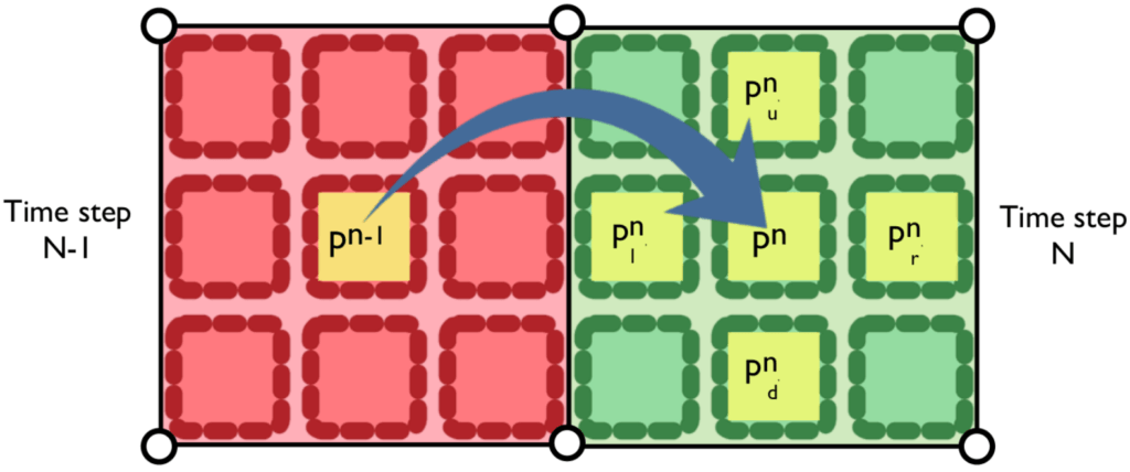
This decouples read and write operations and saves the day, cos everything can safely happen in parallel!
Let’s have a closer look. The first step of the algorithm, the reading of the current values [the yellow squares on the green side of figure 0], can be recklessly parallelized, since portion N of the texture is not changed. The writing process is not a problem either; each parallel thread modifies only the local fragment on portion N-1 [the yellow square in the red side of figure 0], allowing this process to happen concurrently on each point.

Before diving into the code, it’s good to have clear in mind how this can be done in OpenGL.
From OpenGL 4.5, we can “easily” update [render] a fragment of a texture while reading [sampling] another texture portion, as long as the latter is not rendered. We need to set up an FBO to read from and write to the same texture, in a kind of bizarre way.
These are the required steps:

define an FBO that renders to our texture
define two adjacent quads [sets of 4 co-planar vertices], where to place the two portions of the texture [these vertices are showed as 6 white dots in figure 0 – 2 couples are overlapped]
add to each vertex the coordinates of the current texture fragment [p^n-1 in the figure 0] and the coordinates to read the 5 fragments on the opposite texture portion [pⁿ and p_u,d,l,rⁿin figure 0] —> the figure refers only to the texture coordinates needed by the left texture portion; the right case is analogous, in the opposite direction
make successive FBO draw calls alternatively passing the first quad [left texture portion] and the second quad [right texture portion]

Finally, how about the output audio stream?
We could hypothetically sample the texture from the CPU at every simulation step, but this would not work in real-time, cos reading from the video memory takes a lot of time. The solution is to save the audio sample at each step into a buffer in video memory and then read it from the CPU only once every audio callback. It sounds easy, but this approach requires the definition of an extra texture portion, a single pixel line on top of the whole texture where to save the audio output, like an audio buffer. If we couple it to another thin quad, we can update it by calling the same FBO at each simulation step; the update will simply copy the pressure value taken from a chosen domain point/texture fragment [called listener point], a fairly lightweight operation. At this point, we can sample this texture portion once in a while from the CPU and copy its content in the audio buffer directed to the audio card, without excessively affecting the overall performance of the system.
The final texture/quad layout is showed in figure 1:

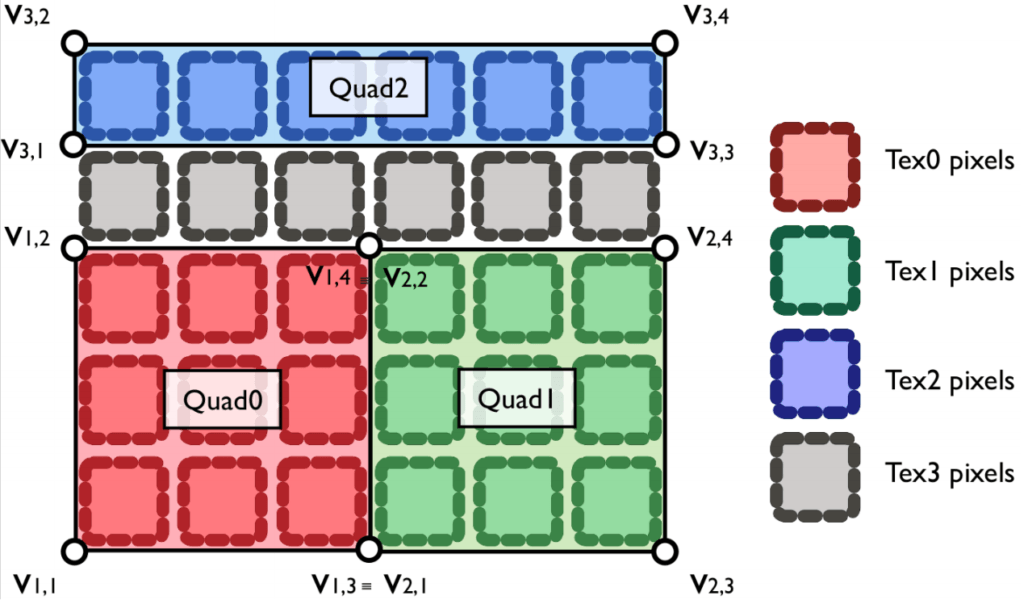
As you can see, there is a further texture portion [in grey in figure 1]. This is a simple separator, with empty/black fragments, that is needed to prevent the neighbor sampling of the topmost fragments of the domain from sampling as top neighbors the audio fragment values. This portion is not coupled with any quad/vertices and is never updated with draw calls. The combination of this extra texture portion plus the audio texture [2 lines of pixels on top of each other] we’ll be referred to as “ceiling”.

Fantastic, we have defined a super cool structure to access and modify all the data needed to our FDTD solver, but I spent no words on its mathematical implementation [i.e., how to update a pressure point]! For sake of simplicity and mental order, this stuff will be described in the next episode (:

//—————————————————————————————————————————————————–
Now let’s delve into the CODE
//—————————————————————————————————————————————————–
The whole project makes use of the glfw3 library, which is one of the most convenient OpenGL libs you can find out there. Hence, the top of the main file looks like this:

 
#include <cstdio>   // always useful (:
#include <cstring> // memset

#include <GL/glew.h>    // basic graphics lib
#include <GLFW/glfw3.h> // GLFW helper library

#include "openGL_functions.h" // wrappers' declarations

#include <cstdio> // always useful (:

#include <cstring> // memset

#include <GL/glew.h> // basic graphics lib

#include <GLFW/glfw3.h> // GLFW helper library

#include "openGL_functions.h" // wrappers' declarations

If you have troubles installing the libs on your machine, you might find a fix in Episode 3, at least for Linux. Another good source is Dr. Anton Gerdelan’s C-OpenGL tutorials.
We understood the physical model and we have a plan on how to run it in OpenGL, so let’s start the implementation. We have to initialize in C++ the OpenGL structures we’re gonna use.

Trivially, the first thing we want to create is a window tied to an OpenGL context and then load the two shader programs we are gonna need, one to render using the FBO, the other to render to screen.
[The following code can be carelessly put inside a big, inelegant main function]

 
int domainSize[2] = {80, 80}; // number of simulation points
float magnifier = 10;
GLFWwindow* window = initOpenGL(domainSize[0], domainSize[1], "My window's name", magnifier);

// where shaders are
const char* vertex_path_fbo      = {"shaders_FDTD/fbo_vs.glsl"}; // vertex shader of solver program
const char* fragment_path_fbo    = {"shaders_FDTD/fbo_fs.glsl"}; // fragment shader of solver program
const char* vertex_path_render   = {"shaders_FDTD/render_vs.glsl"}; // vertex shader of render program
const char* fragment_path_render = {"shaders_FDTD/render_fs.glsl"}; // fragment shader of render program


// FBO shader program [solver]
GLuint shader_program_fbo = 0;
if(!loadShaderProgram(vertex_path_fbo, fragment_path_fbo, vs_fbo, fs_fbo, shader_program_fbo))
	return;


// screen shader program [render]
GLuint shader_program_render = 0;
if(!loadShaderProgram(vertex_path_render, fragment_path_render, vs_render, fs_render, shader_program_render))
	return;

int domainSize[2] = {80, 80}; // number of simulation points

float magnifier = 10;

GLFWwindow* window = initOpenGL(domainSize[0], domainSize[1], "My window's name", magnifier);

// where shaders are

const char* vertex_path_fbo = {"shaders_FDTD/fbo_vs.glsl"}; // vertex shader of solver program

const char* fragment_path_fbo = {"shaders_FDTD/fbo_fs.glsl"}; // fragment shader of solver program

const char* vertex_path_render = {"shaders_FDTD/render_vs.glsl"}; // vertex shader of render program

const char* fragment_path_render = {"shaders_FDTD/render_fs.glsl"}; // fragment shader of render program

// FBO shader program [solver]

GLuint shader_program_fbo = 0;

if(!loadShaderProgram(vertex_path_fbo, fragment_path_fbo, vs_fbo, fs_fbo, shader_program_fbo))

return;

// screen shader program [render]

GLuint shader_program_render = 0;

if(!loadShaderProgram(vertex_path_render, fragment_path_render, vs_render, fs_render, shader_program_render))

return;

The used wrapper functions are declared in openGL_functions.h as follows:

 
GLFWwindow * initOpenGL(int width, int heigth, std::string windowName, float magnifier);
bool loadShaderProgram(const char *vertShaderPath, const char *fragShaderPath, GLuint &vs, GLuint &fs, GLuint &shader_program);

GLFWwindow * initOpenGL(int width, int heigth, std::string windowName, float magnifier);

bool loadShaderProgram(const char *vertShaderPath, const char *fragShaderPath, GLuint &vs, GLuint &fs, GLuint &shader_program);

The window should be as big as the domain, but what’s magnifier? As explained before, in our implementation each grid point basically is a fragment on the texture. By default, when we render the texture on its quad, each fragment becomes a pixel. Given the typical resolution of modern GPUs, this translates into a TINY window! So we use a magnifier as a multiplier factor to stretch the window, so that each fragment can be represented by more pixels. Same domain resolution, nothing magic, just a bigger visualization and slightly more intense rendering process.
In the code I interchangeably use the terms “fragment” and “pixel”, despite this small eventual difference.

The function initOpenGL(…) is quite self explanatory, it creates the window and the context. The only important thing to remark is the fact that it disables V-Sync, so that the screen render does not have to wait for the refresh rate of the display, which would cause several buffer underruns.

With loadShaderProgram(…) we compile the 2 couples of vertex and fragment shaders we want to use for our FBO and screen rendering. The shaders are simple textual files [more info in Episode 3].

And here comes the tough part, the implementation of the 3 quads represented in figure 1.
This means defining an array of vertices [their positions] in that specific layout
BUT
which also contains the texture coordinates showed in figure 0!

avoid to include among the texture coordinates the one related to the local previous pressure value p^n-1[more detailed explanation in the section about the texture initialization].

 
#define NUM_OF_TIMESTEPS 2

/*
 *   full quad/texture layout
 *   _______________________
 *  |_______________________|<----quad2, audio row
 *  |_______________________|<----isolation row, empty
 *  |           |           |              ^
 *  |           |           |       layout "ceiling"
 *  |   quad0   |   quad1   |
 *  |           |           |
 *  |___________|___________|
 *
 */

int clng = 2; // audio row [quad2, at the very top of texture] + isolation row [below audio row] = the "ceiling" of the layout


//-----------------------------------------------------------
// vertices and their attributes
//-----------------------------------------------------------
int numOfAttrElementsPerVertex = 12; // each vertex comes with a set of info, regarding its position and the texture coordinates it can have access to
// these data will be passed to the shader every time there is a draw command, but grouped as attribute arrays
// first we define all the elements of these arrays as a long list
// later we will group them
// the elements' list:
// 2 elements that describe the position of the vertex on the viewport at step N+1 [current quad]
// 		pos x y
// 2 elements that describe the coordinate on the texture associated to the vertex, but at step N [previous quad]
// 		texture coordinate central x y
// 8 elements that describe the neighbor texture coordinates associated to the vertex, but at step N [previous quad]
// 		texture coordinate left x y
// 		texture coordinate up x y
// 		texture coordinate right x y
// 		texture coordinate down x y

// we draw quads, each composed of 4 vertices [each coming with the aforementioned 12 elements]
int numOfVerticesPerQuad = 4; // vertices are grouped in quartets, in a VERY SPECIFIC order:
// bottom left
// top left
// bottom right
// top right
// using this order we can draw a quad passing ONLY 4 VERTICES
// any other order would not work and would oblige us to use 6 VERTICES!
// this is really important to optimize the drawing cycle


// we're gonna set the texture coordinates, so let's calculate how big the texture needs to be
int textureWidth  = domainSize[0]*NUM_OF_TIMESTEPS; // the texture will contain the 2 main quads [quad0 and quad1] side by side
int textureHeight = domainSize[1]+clng; // the texture will stack the main quads, an empty isolation row and the audio row [quad2] ---> see layout diagram towards the top of this file

// now we fill the elements required per each vertex [which later will become attributes]
// the frame of reference for positions is in the center of the texture and coordinates go from -1.0 to 1.0, on both axis
// the frame of reference for texture coords is in the bottom left corner of the texture and coordinates go from 0.0 to 1.0, on both axis
// it's madness, i know, but it's OpenGL

// these are the deltas to compute the texture coordinates of neighbors [tex left, tex up, tex, right, tex down] AKA width and height of fragments
float dx = 1.0/(float)textureWidth;
float dy = 1.0/(float)textureHeight; // this is also combined with clng to make space for audio row and isolation row

// this is the delta to compute the vertex y positions so that we have space for audio row and isolation row
float dy_v = 2.0/(float)textureHeight;

float all_attributes[] = {
	// quad0 [left quadrant]
	// 4 vertices
	// pos N+1/-1		tex C coord N		tex L coord N		tex U coord N		tex R coord N		tex D coord N
	-1, -1,				0.5f, 0,			0.5f-dx, 0,			0.5f, 0+dy,			0.5f+dx, 0,			0.5f, 0-dy,         // bottom left
	-1, 1-clng*dy_v,	0.5f, 1-clng*dy,	0.5f-dx, 1-clng*dy,	0.5f, 1+dy-clng*dy,	0.5f+dx, 1-clng*dy,	0.5f, 1-dy-clng*dy, // top left [leaving space for clng]
	0, -1,				1.0f, 0,			1-dx,    0,			1,    0+dy,			1+dx,    0,			1, 	  0-dy,         // bottom right
	0, 1-clng*dy_v,		1.0f, 1-clng*dy,	1-dx,    1-clng*dy,	1,    1+dy-clng*dy,	1+dx,    1-clng*dy,	1, 	  1-dy-clng*dy, // top right [leaving space for clng]

	// quad1 [right quadrant]
	// 4 vertices
	// pos N+1/-1		tex C coord N		tex L coord N		tex U coord N		tex R coord N		tex D coord N
	0, -1,				0,    0,			0-dx,    0,			0, 	  0+dy,			0+dx,    0,			0,    0-dy,         // bottom left
	0, 1-clng*dy_v,	    0,    1-clng*dy,	0-dx, 	 1-clng*dy,	0,    1+dy-clng*dy,	0+dx,    1-clng*dy,	0,    1-dy-clng*dy, // top left [leaving space for clng]
	1, -1,				0.5f, 0,			0.5f-dx, 0,			0.5f, 0+dy,			0.5f+dx, 0,			0.5f, 0-dy,         // bottom right
	1, 1-clng*dy_v,		0.5f, 1-clng*dy,	0.5f-dx, 1-clng*dy,	0.5f, 1+dy-clng*dy,	0.5f+dx, 1-clng*dy,	0.5f, 1-dy-clng*dy, // top right [leaving space for clng]

	// quad2 [ audio quadrant]
	// 4 vertices
	// pos [no concept of time step]		tex C coords are the only ones required...
	-1, 1-dy_v,			0,    1-dy,			0,    0,			0,    0,			0,    0,			0,    0, // bottom left [1 pixel below top]
	-1, 1,	    		0,    1,			0,    0,			0,    0,			0,    0,			0,    0, // top left
	1, 1-dy_v,			1,    1-dy,			0,    0,			0,    0,			0,    0,			0,    0, // bottom right [1 pixel below top]
	1, 1,				1,    1,			0,    0,			0,    0,			0,    0,			0,    0, // top right
};
// the cool thing is that we give elements for only the extremes of each quad, which will be than correctly replicated
// for any pixel that lies inside these extremes!

#define NUM_OF_TIMESTEPS 2

* full quad/texture layout

* _______________________

* |_______________________|<----quad2, audio row

* |_______________________|<----isolation row, empty

* | | | ^

* | | | layout "ceiling"

* | quad0 | quad1 |

* | | |

* |___________|___________|

int clng = 2; // audio row [quad2, at the very top of texture] + isolation row [below audio row] = the "ceiling" of the layout

//-----------------------------------------------------------

// vertices and their attributes

//-----------------------------------------------------------

int numOfAttrElementsPerVertex = 12; // each vertex comes with a set of info, regarding its position and the texture coordinates it can have access to

// these data will be passed to the shader every time there is a draw command, but grouped as attribute arrays

// first we define all the elements of these arrays as a long list

// later we will group them

// the elements' list:

// 2 elements that describe the position of the vertex on the viewport at step N+1 [current quad]

// pos x y

// 2 elements that describe the coordinate on the texture associated to the vertex, but at step N [previous quad]

// texture coordinate central x y

// 8 elements that describe the neighbor texture coordinates associated to the vertex, but at step N [previous quad]

// texture coordinate left x y

// texture coordinate up x y

// texture coordinate right x y

// texture coordinate down x y

// we draw quads, each composed of 4 vertices [each coming with the aforementioned 12 elements]

int numOfVerticesPerQuad = 4; // vertices are grouped in quartets, in a VERY SPECIFIC order:

// bottom left

// top left

// bottom right

// top right

// using this order we can draw a quad passing ONLY 4 VERTICES

// any other order would not work and would oblige us to use 6 VERTICES!

// this is really important to optimize the drawing cycle

// we're gonna set the texture coordinates, so let's calculate how big the texture needs to be

int textureWidth = domainSize[0]*NUM_OF_TIMESTEPS; // the texture will contain the 2 main quads [quad0 and quad1] side by side

int textureHeight = domainSize[1]+clng; // the texture will stack the main quads, an empty isolation row and the audio row [quad2] ---> see layout diagram towards the top of this file

// now we fill the elements required per each vertex [which later will become attributes]

// the frame of reference for positions is in the center of the texture and coordinates go from -1.0 to 1.0, on both axis

// the frame of reference for texture coords is in the bottom left corner of the texture and coordinates go from 0.0 to 1.0, on both axis

// it's madness, i know, but it's OpenGL

// these are the deltas to compute the texture coordinates of neighbors [tex left, tex up, tex, right, tex down] AKA width and height of fragments

float dx = 1.0/(float)textureWidth;

float dy = 1.0/(float)textureHeight; // this is also combined with clng to make space for audio row and isolation row

// this is the delta to compute the vertex y positions so that we have space for audio row and isolation row

float dy_v = 2.0/(float)textureHeight;

float all_attributes[] = {

// quad0 [left quadrant]

// 4 vertices

// pos N+1/-1 tex C coord N tex L coord N tex U coord N tex R coord N tex D coord N

-1, -1, 0.5f, 0, 0.5f-dx, 0, 0.5f, 0+dy, 0.5f+dx, 0, 0.5f, 0-dy, // bottom left

-1, 1-clng*dy_v, 0.5f, 1-clng*dy, 0.5f-dx, 1-clng*dy, 0.5f, 1+dy-clng*dy, 0.5f+dx, 1-clng*dy, 0.5f, 1-dy-clng*dy, // top left [leaving space for clng]

0, -1, 1.0f, 0, 1-dx, 0, 1, 0+dy, 1+dx, 0, 1, 0-dy, // bottom right

0, 1-clng*dy_v, 1.0f, 1-clng*dy, 1-dx, 1-clng*dy, 1, 1+dy-clng*dy, 1+dx, 1-clng*dy, 1, 1-dy-clng*dy, // top right [leaving space for clng]

// quad1 [right quadrant]

// 4 vertices

// pos N+1/-1 tex C coord N tex L coord N tex U coord N tex R coord N tex D coord N

0, -1, 0, 0, 0-dx, 0, 0, 0+dy, 0+dx, 0, 0, 0-dy, // bottom left

0, 1-clng*dy_v, 0, 1-clng*dy, 0-dx, 1-clng*dy, 0, 1+dy-clng*dy, 0+dx, 1-clng*dy, 0, 1-dy-clng*dy, // top left [leaving space for clng]

1, -1, 0.5f, 0, 0.5f-dx, 0, 0.5f, 0+dy, 0.5f+dx, 0, 0.5f, 0-dy, // bottom right

1, 1-clng*dy_v, 0.5f, 1-clng*dy, 0.5f-dx, 1-clng*dy, 0.5f, 1+dy-clng*dy, 0.5f+dx, 1-clng*dy, 0.5f, 1-dy-clng*dy, // top right [leaving space for clng]

// quad2 [ audio quadrant]

// 4 vertices

// pos [no concept of time step] tex C coords are the only ones required...

-1, 1-dy_v, 0, 1-dy, 0, 0, 0, 0, 0, 0, 0, 0, // bottom left [1 pixel below top]

-1, 1, 0, 1, 0, 0, 0, 0, 0, 0, 0, 0, // top left

1, 1-dy_v, 1, 1-dy, 0, 0, 0, 0, 0, 0, 0, 0, // bottom right [1 pixel below top]

1, 1, 1, 1, 0, 0, 0, 0, 0, 0, 0, 0, // top right

};

// the cool thing is that we give elements for only the extremes of each quad, which will be than correctly replicated

// for any pixel that lies inside these extremes!

We also separatetly save the indices of the two main quads:

 
// this is list of vertices we're gonna draw
// since we'll work on only one quad at the time, we organized their vertices in 2 separate arrays

int vertices[NUM_OF_TIMESTEPS+1][2]; // vertices and attributes will be stored here, for quad0, quad1 and quad2 [2 time steps + audio]

// quad0 is composed of vertices 0 to 3
vertices[0][0] = 0; // index of first vertex
vertices[0][1] = numOfVerticesPerQuad; // number of vertices

// quad1 is composed of vertices 4 to 7
vertices[1][0] = 4;
vertices[1][1] = numOfVerticesPerQuad;

// quad2 is composed of vertices 8 to 11
vertices[2][0] = 8;
vertices[2][1] = numOfVerticesPerQuad;

// this is list of vertices we're gonna draw

// since we'll work on only one quad at the time, we organized their vertices in 2 separate arrays

int vertices[NUM_OF_TIMESTEPS+1][2]; // vertices and attributes will be stored here, for quad0, quad1 and quad2 [2 time steps + audio]

// quad0 is composed of vertices 0 to 3

vertices[0][0] = 0; // index of first vertex

vertices[0][1] = numOfVerticesPerQuad; // number of vertices

// quad1 is composed of vertices 4 to 7

vertices[1][0] = 4;

vertices[1][1] = numOfVerticesPerQuad;

// quad2 is composed of vertices 8 to 11

vertices[2][0] = 8;

vertices[2][1] = numOfVerticesPerQuad;

We will use vertices[][] to alternatively draw the two main quads within the simulation cycle, covered in the next episode.

Then, we pass all the attributes to the VBO and properly set up the VAO, so that the shaders can distinguish vertices’ positions and texture coordinates:

 
//-----------------------------------------------------------
// Vertex Buffer Object, to pass data to graphics card [in our case, they're positions]
//-----------------------------------------------------------
setUpVbo(sizeof (all_attributes), all_attributes, vbo);



//-----------------------------------------------------------
// Vertex Attribute Object, tells the shader how to interpret the VBO's content [vertices and in attributes]
//-----------------------------------------------------------
setUpVao(vbo, vao);

// we pack 2 coordinates [vec2 + vec2] in each attribute [fast]
int numOfElementsPerAttr = 4; // so each attribute will have 4 elements [vec4], taken from the vertices data structure!


// we need 3 attributes to group 12 elements in quartets
// all these 3 attributes must be declared at least in one of the shaders in the program

// we search for them in the FBO, cos it uses all of them [the render shader uses only 1]

// per each attribute we go through all the vertices data structure and extract the 12 elements that we need
// grouping them in 3 vec4

// 0 contains pos [vec2] and texc [vec2]
GLint pos_and_texc_loc = glGetAttribLocation(shader_program_fbo, "pos_and_texc");
glEnableVertexAttribArray(pos_and_texc_loc);
//                     attribute location   4 float elements                           access stride between vertices             elements to skip
glVertexAttribPointer (pos_and_texc_loc, numOfElementsPerAttr, GL_FLOAT, GL_FALSE, numOfAttrElementsPerVertex * sizeof(GLfloat), (void*)(0*numOfElementsPerAttr * sizeof(GLfloat)));

// 1 contains texl [vec2] and texu [vec2]
GLint texl_and_texu_loc = glGetAttribLocation(shader_program_fbo, "texl_and_texu");
glEnableVertexAttribArray(texl_and_texu_loc);
glVertexAttribPointer (texl_and_texu_loc, numOfElementsPerAttr, GL_FLOAT, GL_FALSE, numOfAttrElementsPerVertex * sizeof(GLfloat), (void*)(1*numOfElementsPerAttr * sizeof(GLfloat)));

// 2 contains texr [vec2] and texrd [vec2]
GLint texr_and_texd_loc = glGetAttribLocation(shader_program_fbo, "texr_and_texd");
glEnableVertexAttribArray(texr_and_texd_loc);
glVertexAttribPointer (texr_and_texd_loc, numOfElementsPerAttr, GL_FLOAT, GL_FALSE, numOfAttrElementsPerVertex * sizeof(GLfloat), (void*)(2*numOfElementsPerAttr * sizeof(GLfloat)));

// the attributes are shared between the 2 programs, so once they are successfully initialized
// the render shader will automatically have its own subset working

//-----------------------------------------------------------

// Vertex Buffer Object, to pass data to graphics card [in our case, they're positions]

//-----------------------------------------------------------

setUpVbo(sizeof (all_attributes), all_attributes, vbo);

//-----------------------------------------------------------

// Vertex Attribute Object, tells the shader how to interpret the VBO's content [vertices and in attributes]

//-----------------------------------------------------------

setUpVao(vbo, vao);

// we pack 2 coordinates [vec2 + vec2] in each attribute [fast]

int numOfElementsPerAttr = 4; // so each attribute will have 4 elements [vec4], taken from the vertices data structure!

// we need 3 attributes to group 12 elements in quartets

// all these 3 attributes must be declared at least in one of the shaders in the program

// we search for them in the FBO, cos it uses all of them [the render shader uses only 1]

// per each attribute we go through all the vertices data structure and extract the 12 elements that we need

// grouping them in 3 vec4

// 0 contains pos [vec2] and texc [vec2]

GLint pos_and_texc_loc = glGetAttribLocation(shader_program_fbo, "pos_and_texc");

glEnableVertexAttribArray(pos_and_texc_loc);

// attribute location 4 float elements access stride between vertices elements to skip

glVertexAttribPointer (pos_and_texc_loc, numOfElementsPerAttr, GL_FLOAT, GL_FALSE, numOfAttrElementsPerVertex * sizeof(GLfloat), (void*)(0*numOfElementsPerAttr * sizeof(GLfloat)));

// 1 contains texl [vec2] and texu [vec2]

GLint texl_and_texu_loc = glGetAttribLocation(shader_program_fbo, "texl_and_texu");

glEnableVertexAttribArray(texl_and_texu_loc);

glVertexAttribPointer (texl_and_texu_loc, numOfElementsPerAttr, GL_FLOAT, GL_FALSE, numOfAttrElementsPerVertex * sizeof(GLfloat), (void*)(1*numOfElementsPerAttr * sizeof(GLfloat)));

// 2 contains texr [vec2] and texrd [vec2]

GLint texr_and_texd_loc = glGetAttribLocation(shader_program_fbo, "texr_and_texd");

glEnableVertexAttribArray(texr_and_texd_loc);

glVertexAttribPointer (texr_and_texd_loc, numOfElementsPerAttr, GL_FLOAT, GL_FALSE, numOfAttrElementsPerVertex * sizeof(GLfloat), (void*)(2*numOfElementsPerAttr * sizeof(GLfloat)));

// the attributes are shared between the 2 programs, so once they are successfully initialized

// the render shader will automatically have its own subset working

The used wrapper functions from openGL_functions.h:

 
void setUpVbo(int size, float *vertices, GLuint &vbo);
void setUpVao(GLuint vbo, GLuint &vao);

void setUpVbo(int size, float *vertices, GLuint &vbo);

void setUpVao(GLuint vbo, GLuint &vao);

We move on to the initialization texture. The texture is supposed to contain two copies of the domain and two empty rows of fragments on top.
We first allocate and initialize in CPU memory a flattened multidimensional float array that can contain all the fragments [RGBA channels] we’ll use to fill the texture:

 
//--------------------------------------------------------
// texture pixels
//--------------------------------------------------------
// texturePixels contains all the points [2 quads], starting from left bottom corner
float *texturePixels = new float[textureWidth*textureHeight*4]; // 4 channels per pixel, RGBA
// R channel contains current pressure value
// G channel contains previous pressure value
// B channel defines if the point is boundary [0] or regular [1] --> beta term
// A channel defines if the point receives external excitation [1] or not [0]

// wipe all pixels
memset(texturePixels, 0, sizeof(float)*textureWidth*textureHeight*4);

//--------------------------------------------------------

// texture pixels

//--------------------------------------------------------

// texturePixels contains all the points [2 quads], starting from left bottom corner

float *texturePixels = new float[textureWidth*textureHeight*4]; // 4 channels per pixel, RGBA

// R channel contains current pressure value

// G channel contains previous pressure value

// B channel defines if the point is boundary [0] or regular [1] --> beta term

// A channel defines if the point receives external excitation [1] or not [0]

// wipe all pixels

memset(texturePixels, 0, sizeof(float)*textureWidth*textureHeight*4);

What’s with that previous pressure? We need two channels only to define the type of the local point [B and A], while the R channel is used to store the current pressure. This allows us to reserve the G channel to the storage of the previous local pressure value! Basically, instead of retrieving the previous value from the texture, at every cycle we save a copy in the fragment’s channel, which is always readily accessible. This is quite cool, it can be implemented directly in the shader [next episode] and makes possible to reduce the number of texture coordinates passed along with every vertex position, as mentioned in the section about the used attributes, saving up some memory.
We can do this only because we have a spare channel though! When implementing other FDTD solvers [e.g., implicit] or other physical models we might not have this luxury…indeed we often run short of channels. In those cases, the fallback plan is to simply line up the texture coordinate with the other attributes, as originally conceived.

Once texturePixels[] is allocated, we can focus on the actual domain. The domain is just a portion of the whole texture with pixels carrying particular B and A channel values [beta and excitation terms] that define regular points, boundaries and excitation. We can build it from the CPU side, by simply using a two-dimensional array each containing 2 values for the B and A channel values [so 3 dimensions in total]. The domain we are gonna use is totally empty [regular points], except for a rim of boundary points that surrounds it and an arbitrary excitation point:

 
// domain points' types [same for each quad], from left bottom corner
float **pointType[3];
pointType[0] = new float *[domainSize[0]]; // beta
pointType[1] = new float *[domainSize[0]]; // excitation
for(int i=0; i<domainSize[0]; i++) {
	pointType[0][i] = new float[domainSize[1]];
	pointType[1][i] = new float[domainSize[1]];

	// we init them
	for(int j=0; j<domainSize[1]; j++) {
		pointType[0][i][j] = 1; // regular point beta
		pointType[1][i][j] = 0; // no excitation

		// we also place the excitation point
		if( (i==excitationPos[0]) && (j==excitationPos[1]) )
			pointType[1][i][j] = 1; // excitation
	}
}

// then we add two columns of boundary points, at right and left of domain
for(int i=0; i<domainSize[0]; i++) {
	pointType[0][i][0] = 0; // we only change beta, the transmission value
	pointType[0][i][domainSize[1]-1] = 0;
}
// and finally we add two boundary rows, at top and bottom of domain [they intersect with the columns on the corners]
for(int j=1; j<domainSize[1]-1; j++) {
	pointType[0][0][j] = 0;
	pointType[0][domainSize[0]-1][j] = 0;
}

// domain points' types [same for each quad], from left bottom corner

float **pointType[3];

pointType[0] = new float *[domainSize[0]]; // beta

pointType[1] = new float *[domainSize[0]]; // excitation

for(int i=0; i<domainSize[0]; i++) {

pointType[0][i] = new float[domainSize[1]];

pointType[1][i] = new float[domainSize[1]];

// we init them

for(int j=0; j<domainSize[1]; j++) {

pointType[0][i][j] = 1; // regular point beta

pointType[1][i][j] = 0; // no excitation

// we also place the excitation point

if( (i==excitationPos[0]) && (j==excitationPos[1]) )

pointType[1][i][j] = 1; // excitation

}

// then we add two columns of boundary points, at right and left of domain

for(int i=0; i<domainSize[0]; i++) {

pointType[0][i][0] = 0; // we only change beta, the transmission value

pointType[0][i][domainSize[1]-1] = 0;

}

// and finally we add two boundary rows, at top and bottom of domain [they intersect with the columns on the corners]

for(int j=1; j<domainSize[1]-1; j++) {

pointType[0][0][j] = 0;

pointType[0][domainSize[0]-1][j] = 0;

}

We finish with the texture by copying pointType[][][] [the domain] in the first portion of the array of fragments texturePixels[] [the red pixels in figure 1] and then passing everything to the wrapper function that copies these bits in GPU memory, where the actual texture is allocated:

 
// copy domain points' types in texture pixels [in both quads]
for(int i=0; i<textureWidth; i++) {
	for(int j=0; j<textureHeight-clng; j++) {
		// first quad
		if(i<domainSize[0]) {
			texturePixels[(j*textureWidth+i)*4+2] = pointType[0][i][j]; // beta
			texturePixels[(j*textureWidth+i)*4+3] = pointType[1][i][j]; // excitation
		}
		// second quad
		else if(i>=domainSize[0]) {
			// we have to pick the same data as for first quad
			texturePixels[(j*textureWidth+i)*4+2] = pointType[0][i-domainSize[0]][j]; // beta
			texturePixels[(j*textureWidth+i)*4+3] = pointType[1][i-domainSize[0]][j]; // excitation
		}
	}
}

//--------------------------------------------------------
// texture, same for the 2 programs [FBO and render] but used in different ways [FBO: input/output, render: input]
//--------------------------------------------------------
GLuint texture = 0;
setUpTexture(textureWidth, textureHeight, texturePixels, texture);

// copy domain points' types in texture pixels [in both quads]

for(int i=0; i<textureWidth; i++) {

for(int j=0; j<textureHeight-clng; j++) {

// first quad

if(i<domainSize[0]) {

texturePixels[(j*textureWidth+i)*4+2] = pointType[0][i][j]; // beta

texturePixels[(j*textureWidth+i)*4+3] = pointType[1][i][j]; // excitation

}

// second quad

else if(i>=domainSize[0]) {

// we have to pick the same data as for first quad

texturePixels[(j*textureWidth+i)*4+2] = pointType[0][i-domainSize[0]][j]; // beta

texturePixels[(j*textureWidth+i)*4+3] = pointType[1][i-domainSize[0]][j]; // excitation

}

//--------------------------------------------------------

// texture, same for the 2 programs [FBO and render] but used in different ways [FBO: input/output, render: input]

//--------------------------------------------------------

GLuint texture = 0;

setUpTexture(textureWidth, textureHeight, texturePixels, texture);

As stressed out in the comment, in the FBO shader program the texture will be both read and written, in line with the targeted algorithm, while in the render shader we will simply read its content and accordingly draw pixels on screen. The variable texture [not an original name] contains the handler to the actual texture in GPU memory.
This is the prototype of th used wrapper functions from openGL_functions.h:

 
void setUpTexture(int textureWidth, int textureHeight, float *texturePixels, GLuint &texture);

0 1	void setUpTexture(int textureWidth, int textureHeight, float *texturePixels, GLuint &texture);

Next we initialize the FBO and the PBO.

 
//--------------------------------------------------------
// fbo and draw buffer
//--------------------------------------------------------

// the FBO program will use the framebuffer to write on the texture
// the render program use the read from the texture written by the FBO
setUpFbo(texture, fbo);



//--------------------------------------------------------
// pbo, to read from texture
//--------------------------------------------------------
setUpPbo(sizeof(float)*buffer_size, pbo);

//--------------------------------------------------------

// fbo and draw buffer

//--------------------------------------------------------

// the FBO program will use the framebuffer to write on the texture

// the render program use the read from the texture written by the FBO

setUpFbo(texture, fbo);

//--------------------------------------------------------

// pbo, to read from texture

//--------------------------------------------------------

setUpPbo(sizeof(float)*buffer_size, pbo);

The variable buffer_size is the size in samples of the audio buffer.
Here we use these OpenGL wrapper functions:

 
void setUpFbo(GLuint texture, GLuint &fbo);
void setUpPbo(int size, GLuint &pbo);

void setUpFbo(GLuint texture, GLuint &fbo);

void setUpPbo(int size, GLuint &pbo);

The function setUpFbo(…) initializes an FBO that writes to the passed texture [to actually update the new pressure values in the texture].
The function setUpPbo(…) initializes a PBO that we will use to sample the texture from the CPU [to read and pass the samples stored in the upper part of the texture to the audio buffer].
More details about the actual code in the last episode.

We quickly compute some useful values that will be needed by the shaders:

 
// width and height of each fragment...we have calculated them already, to compute texture coordinates
// we change names to make it easier to grasp
deltaCoordX = dx;
deltaCoordY = dy;

// here we compute the texture coordinates of the listener point
// so that the shader can recognize it
float listenerFragCoord[2][2];
// quad 1      reads audio       from quad 0
listenerFragCoord[1][0] = (float)(listenerPos[0]+0.5) / (float)textureWidth;
listenerFragCoord[1][1] = (float)(listenerPos[1]+0.5) / (float)textureHeight;
// quad 0      reads audio       from quad 1
listenerFragCoord[0][0] = (float)(listenerPos[0]+0.5+domainSize[0]) / (float)textureWidth;
listenerFragCoord[0][1] = (float)(listenerPos[1]+0.5) / (float)textureHeight;
// 0.5 is needed for a perfect match of the fragment we want to sample, don't ask too many questions...it's dangerous |:

// width and height of each fragment...we have calculated them already, to compute texture coordinates

// we change names to make it easier to grasp

deltaCoordX = dx;

deltaCoordY = dy;

// here we compute the texture coordinates of the listener point

// so that the shader can recognize it

float listenerFragCoord[2][2];

// quad 1 reads audio from quad 0

listenerFragCoord[1][0] = (float)(listenerPos[0]+0.5) / (float)textureWidth;

listenerFragCoord[1][1] = (float)(listenerPos[1]+0.5) / (float)textureHeight;

// quad 0 reads audio from quad 1

listenerFragCoord[0][0] = (float)(listenerPos[0]+0.5+domainSize[0]) / (float)textureWidth;

listenerFragCoord[0][1] = (float)(listenerPos[1]+0.5) / (float)textureHeight;

// 0.5 is needed for a perfect match of the fragment we want to sample, don't ask too many questions...it's dangerous |:

The variable listenerPos[2] contains the integer coordinates [row and column of the pixel] of the point of the domain from where we want to sample the audio. It can be freely chosen. From this position we extract the coordinates of the corresponding fragment on the texture. It is important to notice that, since there are 2 copies of the domain, listenerFragCoord[2][2] contains 2 different sets of coordinates linked to the same listener position, one on quad0, the other on quad1. Strangely enough, the fragment for quad0 [listenerFragCoord[0]] points to the listener’s location on quad1, while the fragment for quad1 [listenerFragCoord[1]] points to the location on quad0…they are crossed! I will explain the reason for this crossing in the next episode. Sorry for keeping you hanging /:

Then we conclude the initialization with the uniforms, i.e., the variables the CPU can use to send data to the shaders.
We divide unifroms in 2 groups: static and dynamic.
Static uniforms are set only once, at the beginning of the simulation, hence we immediately init them without saving their location; these are typically related to fixed characteristics of the simulation, like the domain size. The dynamic ones are for values that need to be modified within the simulation cycle, like for example the current excitation value; we save location and update them in the loop.
We start with those for the FBO shader program [shader program = combination of passed vertex and fragment shaders]:

 
//--------------------------------------------------------
// uniforms, the shader vars that we can update from the CPU
//--------------------------------------------------------

// for FBO shader
glUseProgram(shader_program_fbo);

//-------------------------------------------
// static uniforms, that we update once, now
2 different sets of coordinates 
// fragments' width
GLuint deltaCoordX_loc =  glGetUniformLocation(shader_program_fbo, "deltaCoordX");
glUniform1f(deltaCoordX_loc, deltaCoordX);

// listener's fragment coordinates [in both simulation quads]
GLuint listenerFragCoord_loc[2];
char name[22];
for(int i=0; i<NUM_OF_TIMESTEPS; i++) {
	sprintf(name, "listenerFragCoord[%d]", i);
	listenerFragCoord_loc[i] = glGetUniformLocation(shader_program_fbo, name);
	glUniform2f(listenerFragCoord_loc[i], listenerFragCoord[i][0], listenerFragCoord[i][1]);
}

//-------------------------------------------
// dynamic uniforms, which we will be updated within the simulation loop

// to tell the shader what to do
state_loc = glGetUniformLocation(shader_program_fbo, "state");

// to pass excitation to excitation points
excitation_loc = glGetUniformLocation(shader_program_fbo, "excitation");

wrCoord_loc = glGetUniformLocation(shader_program_fbo, "wrCoord");

//-------------------------------------------
// texture 

// we say that the uniform called inOutTexture [of type sampler2D] in the FBO shader refers to the texture number zero that we created and initialized
// the FBO will automatically write on it anyway, but doing so we can ALSO READ from it, which is fundamental
glUniform1i(glGetUniformLocation(shader_program_fbo, "inOutTexture"), 0); // we do this only once at the beginning

//--------------------------------------------------------

// uniforms, the shader vars that we can update from the CPU

//--------------------------------------------------------

// for FBO shader

glUseProgram(shader_program_fbo);

//-------------------------------------------

// static uniforms, that we update once, now

2 different sets of coordinates

// fragments' width

GLuint deltaCoordX_loc = glGetUniformLocation(shader_program_fbo, "deltaCoordX");

glUniform1f(deltaCoordX_loc, deltaCoordX);

// listener's fragment coordinates [in both simulation quads]

GLuint listenerFragCoord_loc[2];

char name[22];

for(int i=0; i<NUM_OF_TIMESTEPS; i++) {

sprintf(name, "listenerFragCoord[%d]", i);

listenerFragCoord_loc[i] = glGetUniformLocation(shader_program_fbo, name);

glUniform2f(listenerFragCoord_loc[i], listenerFragCoord[i][0], listenerFragCoord[i][1]);

}

//-------------------------------------------

// dynamic uniforms, which we will be updated within the simulation loop

// to tell the shader what to do

state_loc = glGetUniformLocation(shader_program_fbo, "state");

// to pass excitation to excitation points

excitation_loc = glGetUniformLocation(shader_program_fbo, "excitation");

wrCoord_loc = glGetUniformLocation(shader_program_fbo, "wrCoord");

//-------------------------------------------

// texture

// we say that the uniform called inOutTexture [of type sampler2D] in the FBO shader refers to the texture number zero that we created and initialized

// the FBO will automatically write on it anyway, but doing so we can ALSO READ from it, which is fundamental

glUniform1i(glGetUniformLocation(shader_program_fbo, "inOutTexture"), 0); // we do this only once at the beginning

In the next episode I’ll show how exactly we use these uniforms and why we init the static ones with these values.
The texture uniform (sample2d type) is a case on its own. It is needed to give the FBO shader the capability to read from it [so far it could only write to it]; it is in a sense dynamic, in the sense that it will be constantly changed, but at the same static, since we are not directly updating its values from the CPU [the shader will do that]. Here we are simply initializing it by mapping it to the first texture we created [index 0].

Then same thing for render shader program uniforms:

 
// for render shader
glUseProgram(shader_program_render);

//-------------------------------------------
// static uniforms
GLuint deltaCoord_loc_render =  glGetUniformLocation(shader_program_render, "deltaCoord");
glUniform2f(deltaCoord_loc_render, deltaCoordX, deltaCoordY);

// listener's fragment coordinates [only quad0, cos we only render that one]
GLuint listenerFragCoord_loc_render = glGetUniformLocation(shader_program_render, "listenerFragCoord");
glUniform2f(listenerFragCoord_loc_render, listenerFragCoord[0][0], listenerFragCoord[0][1]);

//-------------------------------------------
// texture
// then we say that the uniform called inputTexture [of type sampler2D] in the render shader refers to the same texture too
glUniform1i(glGetUniformLocation(shader_program_render, "inputTexture"), 0);

glUseProgram(0); // done, we'll re-activate the proper shader program later

// for render shader

glUseProgram(shader_program_render);

//-------------------------------------------

// static uniforms

GLuint deltaCoord_loc_render = glGetUniformLocation(shader_program_render, "deltaCoord");

glUniform2f(deltaCoord_loc_render, deltaCoordX, deltaCoordY);

// listener's fragment coordinates [only quad0, cos we only render that one]

GLuint listenerFragCoord_loc_render = glGetUniformLocation(shader_program_render, "listenerFragCoord");

glUniform2f(listenerFragCoord_loc_render, listenerFragCoord[0][0], listenerFragCoord[0][1]);

//-------------------------------------------

// texture

// then we say that the uniform called inputTexture [of type sampler2D] in the render shader refers to the same texture too

glUniform1i(glGetUniformLocation(shader_program_render, "inputTexture"), 0);

glUseProgram(0); // done, we'll re-activate the proper shader program later

In this case we only have static uniforms, cos the render pass depends exclusively on the pressure values read from the texture and is not influenced by any direct external parameter [see next episode].
The texture itself in this case is accessed only [there is no FBO], as suggested by the name inputTexture. But it is actually the same texture we use with the FBO! It is still indexed as 0 indeed.

THE INITIALIZATION IS DONE.
Whoa!

That’s all for now, stay tuned for the next post:
Episode 2 – Simulation Cycle and Shader Programs [in progress]

Hopefully it will add an important piece to the puzzle and clarify some doubts. It will also contain the full downloadable version of the main.cpp file.
In the meanwhile, always happy to answer questions and correct possible mistakes/imprecision.

later_